-
UID:317649
-
- 注册时间2020-06-19
- 最后登录2026-09-04
- 在线时间1983小时
-
-
访问TA的空间加好友用道具
|
简介:本文是以十字元件为背景光源,经过一个透镜元件成像在探测器上,并显示其热成像图。 J,:&U
wkv t[J=8rhER 成像示意图 Vi: ^bv 首先我们建立十字元件命名为Target $%q=tn'EX %0} ^M1 创建方法: }04mJY[ A$r$g\5+ 面1 : JC%&d1
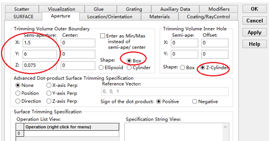
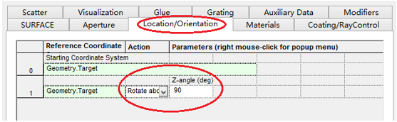
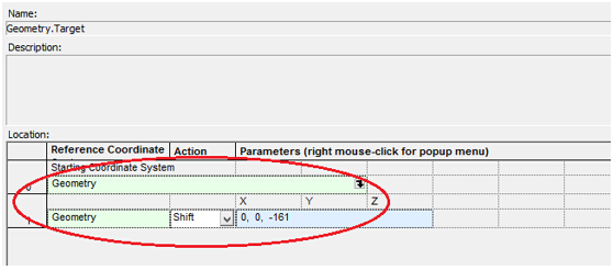
面型:plane /ZD 6pF 材料:Air }rI:pp^KS 孔径:X=1.5, Y=6,Z=0.075,形状选择Box Hc=QSP ('SId@ @`dg:P*[ 辅助数据: G/N c@XG\ 首先在第一行输入temperature :300K, uZtN,Un emissivity:0.1; @U18Dj[ ^L5-2;s<U' n'v\2(&uYN 面2 : z,4mg6gt 面型:plane <|4$TH^t 材料:Air dgF%&*Il]O 孔径:X=1.5, Y=6,Z=0.075,形状选择Box _ Lb"yug #'q7 x 7Vsp<s9bj 位置坐标:绕Z轴旋转90度, i-Rn,}v KF00=HE|] H:]cBk^[, 辅助数据: P2a5<#_| >PSO]%mE 首先在第一行输入temperature :300K,emissivity: 0.1; [p9v#\G; [ s{Y4wvQyB 8{!d'Pks Target 元件距离坐标原点-161mm;
k[D_L` u*G<? o]4\Geg$ 单透镜参数设定:F=100, bend=0, 位置位于坐标原点 uy's eJ Zt!A!Afu lb.Q^TghU 探测器参数设定: OALNZKP b/'c
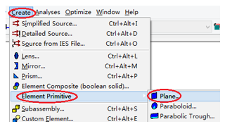
h 在菜单栏中选择Create/Element Primitive /plane ^
*"f C ~2"hh$ hr}f5Z)^v Q2VF+g, 1j$\ 48Z G n]qh(N> 元件半径为20mm*20,mm,距离坐标原点200mm。 CpO_p%P ^PTf8o 光源创建: h6
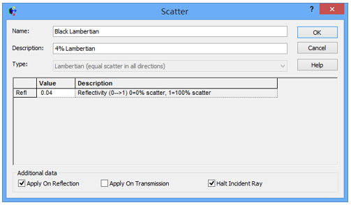
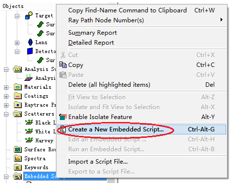
{vbYj Bz/Vzc( 光源类型选择为任意平面,光源半角设定为15度。 &2y4k"B&) cK+TE8ao =Z 我们将光源设定在探测器位置上,具体的原理解释请见本章第二部分。 {siOa%;* aDKb78 1d 我们在位置选项又设定一行的目的是通过脚本自动控制光源在探测器平面不同划分区域内不同位置处追迹光线。 p H y K:a8}w>Up TU0-L35P1 功率数值设定为:P=sin2(theta) theta为光源半角15度。我们为什么要这么设定,在第二部分会给出详细的公式推导。 js<d"m* xmv%O&0^} 创建分析面: ;7lON-@BI wQ/* f9 CJ\a7=*i 到这里元件参数设定完成,现在我们设定元件的光学属性,在前面我们分别对第一和第二面设定的温度和发射系数,散射属性我们设定为黑朗伯,4%的散射。并分别赋予到面一和面二。 a/j;1xcc< bV8+Eu }tW-l*\U 到此,所有的光学结构和属性设定完成,通过光线追迹我们可以查看光线是否可以穿过元件。 L/"};VI *8Z2zmZtR^ FRED在探测器上穿过多个像素点迭代来创建热图 I9S;t_Z< >ou=}/< FRED具有一个内置的可编译的Basic脚本语言。从Visual Basic脚本语言里,几乎所有用户图形界面(GUI)命令是可用这里的。FRED同样具有自动的客户端和服务器能力,它可以被调用和并调用其他可启动程序,如Excel。因此可以在探测器像素点上定义多个离轴光源,及在FRED Basic脚本语言里的For Next loops语句沿着探测器像素点向上和向下扫描来反向追迹光线,这样可以使用三维图表查看器(Tools/Open plot files in 3D chart)调用和查看数据。 32[}@f2q 将如下的代码放置在树形文件夹 Embedded Scripts, m1X7zU Cy @f-X/q]P
e^Zm09J 打开后清空里面的内容,此脚本为通用脚本适用于一切可热成像的应用。 :5NMgR.d hpAdoy[ 绿色字体为说明文字, a;HAuy`M x t )zd'[ '#Language "WWB-COM" xol%\$| 'script for calculating thermal image map %e E^Y<@g 'edited rnp 4 november 2005 9(N 1Z# $X` 'declarations
OUv<a`0 Dim op As T_OPERATION Z+El(f x Dim trm As T_TRIMVOLUME c@t?R$c Dim irrad(32,32) As Double 'make consistent with sampling _Je4&KU Dim temp As Double o+a= Dim emiss As Double
IOl_J>D]F Dim fname As String, fullfilepath As String V.GM$ U**8^:*y#: 'Option Explicit F^yW3|Sb Y !<m8\ Sub Main KZppQ0 'USER INPUTS DK IH{:L7 nx = 31 Cr5ND\ ny = 31 XN df numRays = 1000 u&:N`f minWave = 7 'microns 3oCI1>k maxWave = 11 'microns *
65/gG8> sigma = 5.67e-14 'watts/mm^2/deg k^4 z#tIa fname = "teapotimage.dat" o<Zlm)"%1 ]01`r/->\ Print "" {*yvvb Print "THERMAL IMAGE CALCULATION" _?c.m*)A Q|(}rIWOQA detnode = FindFullName( "Geometry.Detector.Surface" ) '找到探测器平面节点 &6x(%o| <0CjEsAB] Print "found detector array at node " & detnode mU/o%|h V:n0BlZ,B srcnode = FindFullName( "Optical Sources.Source 1" ) '找到光源节点 ?@b6(f
xX `|'w]rj:"+ Print "found differential detector area at node " & srcnode }t)+eSUA tu
-a`h_NJ GetTrimVolume detnode, trm ,h*gd^i detx = trm.xSemiApe n7!T{+ge dety = trm.ySemiApe A,~3oQV area = 4 * detx * dety .|,LBc! Print "detector array semiaperture dimensions are " & detx & " by " & dety YdhTjvx Print "sampling is " & nx & " by " & ny hi8q?4jE f8Hq&_Pn 'reset differential detector area dimensions to be consistent with sampling cE\w6uBR1 pixelx = 2 * detx / nx t<!m4Yd|# pixely = 2 * dety / ny *rq*li; SetSourcePosGridRandom srcnode, pixelx / 2, pixely / 2, numRays, False =6sP`: Print "resetting source dimensions to " & pixelx / 2 & " by " & pixely / 2 7
Lm9I 8+'}` 'reset the source power 'Ea3(OsuXn SetSourcePower( srcnode, Sin(DegToRad(15))^2 ) !l'nX Print "resetting the source power to " & GetSourcePower( srcnode ) & " units"
PL:(Se% gT)(RS`_) 'zero out irradiance array B"4 3o7C For i = 0 To ny - 1 S@qPf0dL< For j = 0 To nx - 1 v$}^$8` irrad(i,j) = 0.0 ,
'pYR]3 Next j zIc6L3w$ Next i =Vg~ VD *l_a=[<[ 'main loop IL@yGuO, EnableTextPrinting( False ) Thggas, 7Jb&~{DVk ypos = dety + pixely / 2 4&*lpl*N For i = 0 To ny - 1 |O8e;v72g^ xpos = -detx - pixelx / 2 0)dpU1B#M ypos = ypos - pixely ]j&m\'-s ^%\a,~ EnableTextPrinting( True ) SgU@`Pb Print i >k
@t.PeoV EnableTextPrinting( False ) iA[T'+.Y
eXl?f_9 c^|8qvS$ For j = 0 To nx - 1 }u^bTR?3 h[(YH ;Y xpos = xpos + pixelx 0]>bNbLB" OS[
s Qo5 'shift source 2-F7tcya| LockOperationUpdates srcnode, True Jk.x^ GetOperation srcnode, 1, op i@/% E~ W op.val1 = xpos ?wtKi#k'v# op.val2 = ypos ]yOM SetOperation srcnode, 1, op m-{DhJV LockOperationUpdates srcnode, False \KV.lG! kHK<~srB 'raytrace 7] y3<t DeleteRays +C=vuR CreateSource srcnode lg|6~=aQ
TraceExisting 'draw i3 js'?7E lr&2,p< 'radiometry ei2?H;H; For k = 0 To GetEntityCount()-1 jnV#Q
; If IsSurface( k ) Then ca=MUm=B temp = AuxDataGetData( k, "temperature" ) Kj0)/Fjl+ emiss = AuxDataGetData( k, "emissivity" ) }%KQrlbHJl If ( temp <> 0 And emiss <> 0 ) Then &tOo[U? ProjSolidAngleByPi = GetSurfIncidentPower( k ) wo9R:kQ frac = BlackBodyFractionalEnergy ( minWave, maxWave, temp ) frbd{o irrad(i,j) = irrad(i,j) + frac * emiss * sigma * temp^4 * ProjSolidAngleByPi -n:2US< End If l"8g9z %\it4 r3 End If +aL6$ 9ERdjS Next k
4H;g"nWqO $bp'b<jx Next j >(:3H+ -Ua5anzB Next i /8Lb_QH{ EnableTextPrinting( True ) f?.}S]u5 0Cc3NNdz 'write out file F]OWqUV fullfilepath = CurDir() & "\" & fname eI|FrBq% Open fullfilepath For Output As #1 li3X} Print #1, "GRID " & nx & " " & ny " "`z3- Print #1, "1e+308" (ht"wY#T<( Print #1, pixelx & " " & pixely $jk4H+H- Print #1, -detx+pixelx/2 & " " & -dety+pixely/2 FUI/ A> L< maxRow = nx - 1 s2sJJdN maxCol = ny - 1 D[T\_3W For rowNum = 0 To maxRow ' begin loop over rows (constant X) @>`N%wH' row = "" 8hV4l'Pa72 For colNum = maxCol To 0 Step -1 ' begin loop over columns (constant Y) L `2{H%J` row = row & irrad(colNum,rowNum) & " " ' append column data to row string d3oRan}z Next colNum ' end loop over columns JA >&$h Sn97DCdk Print #1, row l2#~
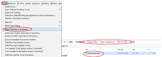
Mf5kknYuL9 Next rowNum ' end loop over rows _576Qa'rm Close #1 N]BH6 7< ({4?RtYm Print "File written: " & fullfilepath pJ?y Print "All done!!" B_!S\?}$ End Sub p@$92> ' sVO|Ghy65 在输出报告中,我们会看到脚本对光源的孔径和功率做了修改,并最终经过31次迭代,将所有的热成像数据以dat的格式放置于: R]Fa?uQW
}m!T~XR</ ~HctXe' x 找到Tools工具,点击Open plot files in 3D chart并找到该文件 x!4<ff. ^(*eo e ~LH).\V 打开后,选择二维平面图: m=`V 'fb&3
|